Agriculture
Wildfire Risk: Forest Fuel Monitor with Sentinel-1 and Sentinel-2
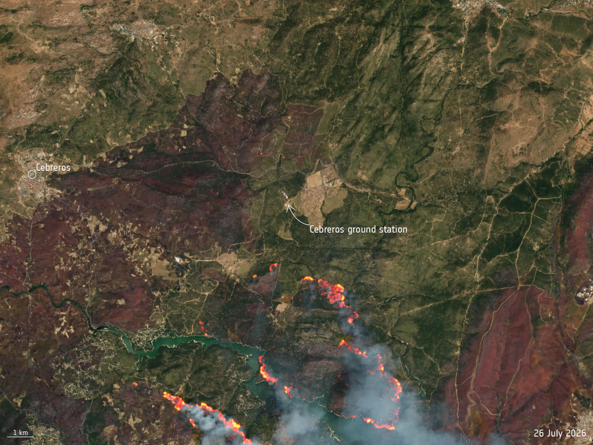
Wildfire risk assessment with remote sensing measures potential fuel. Sentinel-2 shortwave infrared (SWIR) moisture indices track how dry the canopy is, Sentinel-1 Synthetic Aperture Radar (SAR) keeps the record continuous through cloud, and a weather-driven fire danger index supplies the ignition half.
The SWIR moisture indices are band ratios pairing a near-infrared band against a shortwave infrared one, where leaf water absorbs, so the index falls as the canopy dries. Sentinel-1 SAR illuminates the ground with its own C-band microwave signal instead of relying on sunlight, which is why it returns a usable image through cloud and at night. A fire danger index runs temperature, relative humidity, wind and recent rainfall through fuel moisture codes to rate how readily a fire would start and spread on a given day.
But the usefulness is only revealed by its anomaly, not the raw index value. A Normalized Difference Moisture Index (NDMI) of 0.18 means nothing on its own, because a pine stand, a beech stand and a scrub patch sit at different baselines. The same 0.18 in a stand that normally reads 0.34 on that day of year is a two-sigma dryness anomaly. Most of the pipeline below exists to produce that one comparison.
1st: Building the anomaly baseline
Published live fuel moisture content (LFMC) thresholds are ecosystem-specific: Dennison and Moritz (2009) found a critical LFMC near 79% for southern California chaparral, but that cannot be transferred to a Central European spruce stand. Compute each pixel’s departure from its own history instead.
- Pull five years of Sentinel-2 Level-2A: bands B8A, B11, B4, B8 and the Scene Classification Layer (SCL).
- Mask clouds. Drop SCL classes 3 (cloud shadow), 8 and 9 (cloud, medium and high probability) and 10 (thin cirrus), then dilate by two to three pixels.
- Build a per-pixel, per-day-of-year climatology. Median NDMI over observations within a plus or minus 15-day window across the five baseline years, plus median absolute deviation (MAD) for dispersion, which a single unmasked cloud will not blow up.
- Record a fuel type per pixel alongside the baseline. Anomalies are comparable across stands, but their consequence is not: two sigma in flammable shrubland is a different operational fact from two sigma in a riparian broadleaf strip.
The climatology is a one-time heavy job and is where the compute budget goes. Steps 1 to 3 split across two machines: the pixel-heavy reduction runs next to the archive on openEO at the Copernicus Data Space Ecosystem, and the day-of-year statistics run locally on what comes back.
# --- server side: cloud-masked NDMI, reduced to dekadal medians ------------
import numpy as np
import openeo

con = openeo.connect("openeo.dataspace.copernicus.eu").authenticate_oidc()

s2 = con.load_collection(
    "SENTINEL2_L2A",
    spatial_extent=aoi,                       # GeoJSON of the forest management unit
    temporal_extent=["2021-01-01", "2026-08-01"],
    bands=["B8A", "B11", "SCL"],
)

scl = s2.band("SCL")
cloud = (scl == 3) | (scl == 8) | (scl == 9) | (scl == 10)   # shadow, cloud med/high, cirrus
cloud = cloud.apply_kernel(np.ones((5, 5))) > 0              # step 2: dilate ~2 px

ndmi = (s2.band("B8A") - s2.band("B11")) / (s2.band("B8A") + s2.band("B11"))
ndmi = ndmi.mask(cloud)                                      # drops pixels where mask is true

ndmi.aggregate_temporal_period(period="dekad", reducer="median") \
    .execute_batch("ndmi_dekads.nc")          # ~36 slices a year, small enough to pull down
The dekadal cube is a composite, not yet a baseline. Step 3 turns it into one by grouping across years:
# --- local: day-of-year climatology, median and MAD ------------------------
import xarray as xr

cube = xr.open_dataarray("ndmi_dekads.nc")               # dims (t, y, x)
doy = cube.t.dt.dayofyear

def climatology(target_doy, window=15):
    delta = (doy - target_doy + 182) % 365 - 182         # signed circular distance
    w = cube.sel(t=abs(delta) <= window)                 # same season, all five years
    med = w.median("t")
    mad = abs(w - med).median("t")                       # per-pixel MAD
    return med, mad

med_doy, mad_doy = climatology(today.dayofyear)
z = (ndmi_now - med_doy) / (1.4826 * mad_doy)            # the score of stage 2, step 2
Step 4 is not a Sentinel-2 computation at all, which is why it is absent above: fuel type comes from a stand register or a land-cover product, rasterised once onto the same grid with rasterio.features.rasterize and stored beside med_doy and mad_doy.
2nd: Continuous wildfire risk assessment
With the climatology in place, the recurring job runs every 5 to 10 days:
- Composite. A rolling 10 to 20 day median of cloud-free NDMI, not a single scene.
- Score.
z = (NDMI_now - med_doy) / (1.4826 * mad_doy)against that pixel’s baseline for that day of year. A value of -2 then means the same thing in a spruce plantation and an oak stand. - Fill the gaps. When the optical gap passes about 15 days, substitute a Sentinel-1 derived proxy and flag those pixels as SAR-derived so the confidence drop stays visible downstream.
- Gate on fire weather. The Canadian Fire Weather Index (FWI), which the European Forest Fire Information System (EFFIS) publishes for Europe on a roughly 8 km grid, sets the regional alert level; the 20 m anomaly ranks stands inside it. Resampling an 8 km index to 20 m does not give it 20 m structure, so keep the two as separate inputs to a decision table rather than summing them into one raster.
- Emit an ordering, not a binary map: driest stands by anomaly, weighted by fuel load and slope.
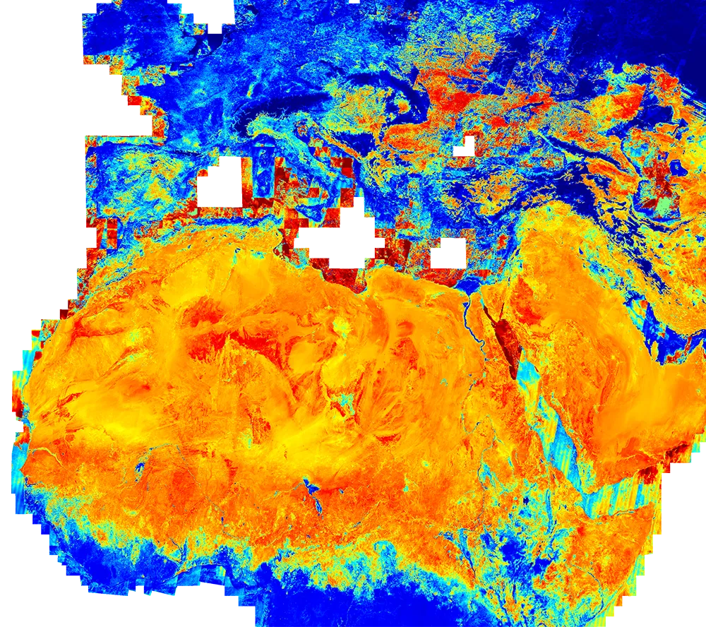 NDMI of northern Africa and Europe, 27.12.2019 SentinelHub
Further details on the relevant Sentinels and Indices
Sentinel-2: thirteen bands, three resolutions
Sentinel-2 is an optical mission flown as a nominal pair, sun-synchronous at 786 km with a 290 km swath, each satellite carrying the MultiSpectral Instrument (MSI). Sentinel-2C launched in September 2024 and replaced Sentinel-2A in primary operations in January 2025, so the operating pair is Sentinel-2B and Sentinel-2C, giving 5 days at the equator against 10 days per satellite. Sentinel-2A has been on a life-extension campaign since March 2025 and adds coverage over Europe and the tropics while it lasts.
The MSI has 13 bands, labelled B1 through B12 by increasing central wavelength, with B8A inserted between B8 and B9 rather than renumbering the rest, so the letters carry position rather than category. The resolution tiers do carry meaning: sharpest optics to the mapping bands, coarser sampling to the atmospheric-correction ones.
| Band | Centre (nm) | Resolution | What it is for |
|---|---|---|---|
| B1 | 443 | 60 m | Aerosol retrieval (atmospheric correction) |
| B2, B3, B4 | 490, 560, 665 | 10 m | Blue, green, red |
| B5, B6, B7 | 705, 740, 783 | 20 m | Red edge, chlorophyll and stress |
| B8 | 833 | 10 m | Wide near infrared (NIR) |
| B8A | 865 | 20 m | Narrow NIR, cleaner of water vapour |
| B9 | 945 | 60 m | Water vapour retrieval |
| B10 | 1375 | 60 m | Cirrus detection (not in surface products) |
| B11 | 1610 | 20 m | Shortwave infrared (SWIR), moisture |
| B12 | 2190 | 20 m | SWIR, moisture and burn severity |
Three of those do the work here: B8 or B8A, B11 and B4.
Leaf water is why. The Remote Sensing review lists liquid water absorption peaks of increasing size at 970, 1200, 1450, 1950 and 2500 nm. Sentinel-2 misses the deep ones, but B11 at 1610 nm and B12 at 2190 nm sit on shoulders strong enough to move a normalized ratio. That is why moisture indices use SWIR, and why the Normalized Difference Vegetation Index (NDVI) is the wrong tool for dryness: it tracks greenness, and a conifer stand can dry to dangerous levels while staying green.
| Index | Formula (Sentinel-2) | What it tracks | Native resolution |
|---|---|---|---|
| NDMI | (B8 - B11) / (B8 + B11) | Canopy water content | 20 m (B11 limits it) |
| NDMI, matched-resolution variant | (B8A - B11) / (B8A + B11) | Canopy water content | 20 m, no resampling |
| Normalized Difference Water Index (NDWI) | (B3 - B8) / (B3 + B8) | Open water, not leaf water | 10 m |
| Normalized Burn Ratio (NBR) | (B8 - B12) / (B8 + B12) | Post-fire severity, not pre-fire risk | 20 m |
| NDVI | (B8 - B4) / (B8 + B4) | Greenness and fuel load, not dryness | 10 m |
The standard NDMI definition in the Sentinel Hub custom scripts library pairs B8 with B11, resampling a 10 m band against a 20 m one; B8A keeps both at native 20 m and avoids an interpolation artefact along stand edges. NDWI is a water-body index despite the name, so substituting it for NDMI produces a map that responds to rivers. NDVI still belongs in the stack as the fuel-load proxy, just not as a dryness signal.
Sentinel-1: radar, so clouds stop mattering
Sentinel-1 carries a C-band Synthetic Aperture Radar at 5.405 GHz, about 5.55 cm wavelength, from a 693 km orbit. Over land the default is Interferometric Wide swath (IW) mode: 250 km swath, 5 by 20 m single-look resolution, dual polarisation VV plus VH.
VV means the radar transmits and receives vertically polarised waves; VH transmits vertically and receives horizontally, which happens when the wave depolarises inside a structured volume such as a canopy. That is why the ratio of the two carries vegetation structure rather than surface brightness.
The reason it is in the stack at all is that a pre-season frontal period, smoke haze or a maritime climate can blank the optical record for a fortnight, often exactly when the data is wanted. It contributes three things. Continuity, in backscatter series with no holes where the clouds were, which is the main reason to add it. Structure, through the dual-polarimetric cross ratio (VH over VV, or the difference in decibels) and the radar vegetation index RVI = 4 * VH / (VV + VH), feeding the fuel-load side. And a moisture signal confounded by soil moisture under and between the canopy, which is why step 3 above treats it as a gap filler rather than a second opinion.
Frequently asked questions
Can satellites detect wildfire risk before a fire starts?
Partly. Satellites measure the fuel side of risk well: how much vegetation is there, how dry it is relative to its own history, and what the terrain looks like. They cannot measure ignition, which the IntechOpen review of remote sensing in wildfires puts at over 90% human-caused in the Mediterranean, and they cannot see surface fuels under a closed canopy. Treat the output as a prioritisation layer feeding a fire danger index.
Which satellite index is best for measuring vegetation dryness?
NDMI, from a near-infrared band and the 1610 nm shortwave infrared band, is the workhorse for canopy water content, because liquid water absorbs strongly in the SWIR. NDVI tracks greenness rather than moisture and can stay high in a dangerously dry conifer stand. NDWI, despite the name, separates open water rather than leaf water. Use NDMI for dryness and NDVI for fuel load.
How often can Sentinel-2 and Sentinel-1 update a fire risk map?
Sentinel-2 has a five-day nominal revisit at the equator with two satellites, but the usable rate depends on cloud, so realistic optical updates run every one to three weeks. Sentinel-1 re-established a six-day repeat cycle in June 2026 with Sentinel-1C and Sentinel-1D, and it observes through cloud, so it bounds the worst case when optical goes blind.
Where do you get Sentinel data for a forest monitoring system?
The Copernicus Data Space Ecosystem provides Sentinel-1 and Sentinel-2 through several interfaces: a STAC (SpatioTemporal Asset Catalog) and OData catalogue for search, an openEO API for server-side processing next to the data, the Sentinel Hub API for rendered and statistical outputs, and OGC web services for GIS clients. Processing next to the archive avoids downloading terabytes for a multi-year baseline.
Can Sentinel-1 SAR measure fuel moisture directly?
Not cleanly. C-band backscatter responds to total water content in the scattering volume, which mixes canopy moisture with soil moisture, and it is also sensitive to incidence angle and terrain. It is a strong continuity and structure layer and a weak direct moisture retrieval. Run optical as the primary signal and fall back to SAR when the optical gap exceeds about 15 days.
Sources and further reading
- Copernicus, Sentinel-2 mission, constellation status and band specifications (SentiWiki)
- Copernicus, Sentinel-1 mission, acquisition modes, polarisation and product levels (SentiWiki)
- Copernicus Data Space Ecosystem, Sentinel-1C/D final orbital configuration achieved, June 2026
- Copernicus Data Space Ecosystem, catalogue, openEO, Sentinel Hub and OGC APIs
- Sentinel Hub, NDMI custom script and band definition
- EFFIS (Copernicus Emergency Management Service), fire danger forecast and Fire Weather Index classes
- Dennison and Moritz, Critical live fuel moisture in chaparral ecosystems, International Journal of Wildland Fire 2009
- Watt et al., Monitoring wildfire risk with a near-real-time live fuel moisture content system: a review and roadmap for operational application in New Zealand, Remote Sensing 17(21) 2025
- Zagalikis, Remote sensing and GIS applications in wildfires, IntechOpen 2023