Real-Time Kinematic: How RTK Works in 5 Steps

Real-time kinematic (RTK) positioning reaches 1 to 2 cm by measuring the carrier wave of Global Navigation Satellite System (GNSS) signals and solving for the whole number of wavelengths to each satellite. A base station at a known point streams its observations; differencing them against the rover’s cancels the shared errors and leaves an integer to search for and verify.

The method is five steps: double-difference, float solution, integer search, validation, and holding the fix through cycle slips. But the last two steps decide whether a position can be trusted, because a wrong integer set still reports “fixed” while sitting decimeters off. Distance from the base is the hard limit, which is why accuracy specs read “1 cm + 1 ppm” (parts per million) and why network RTK and Precise Point Positioning (PPP) exist.

How real-time kinematic works in five steps

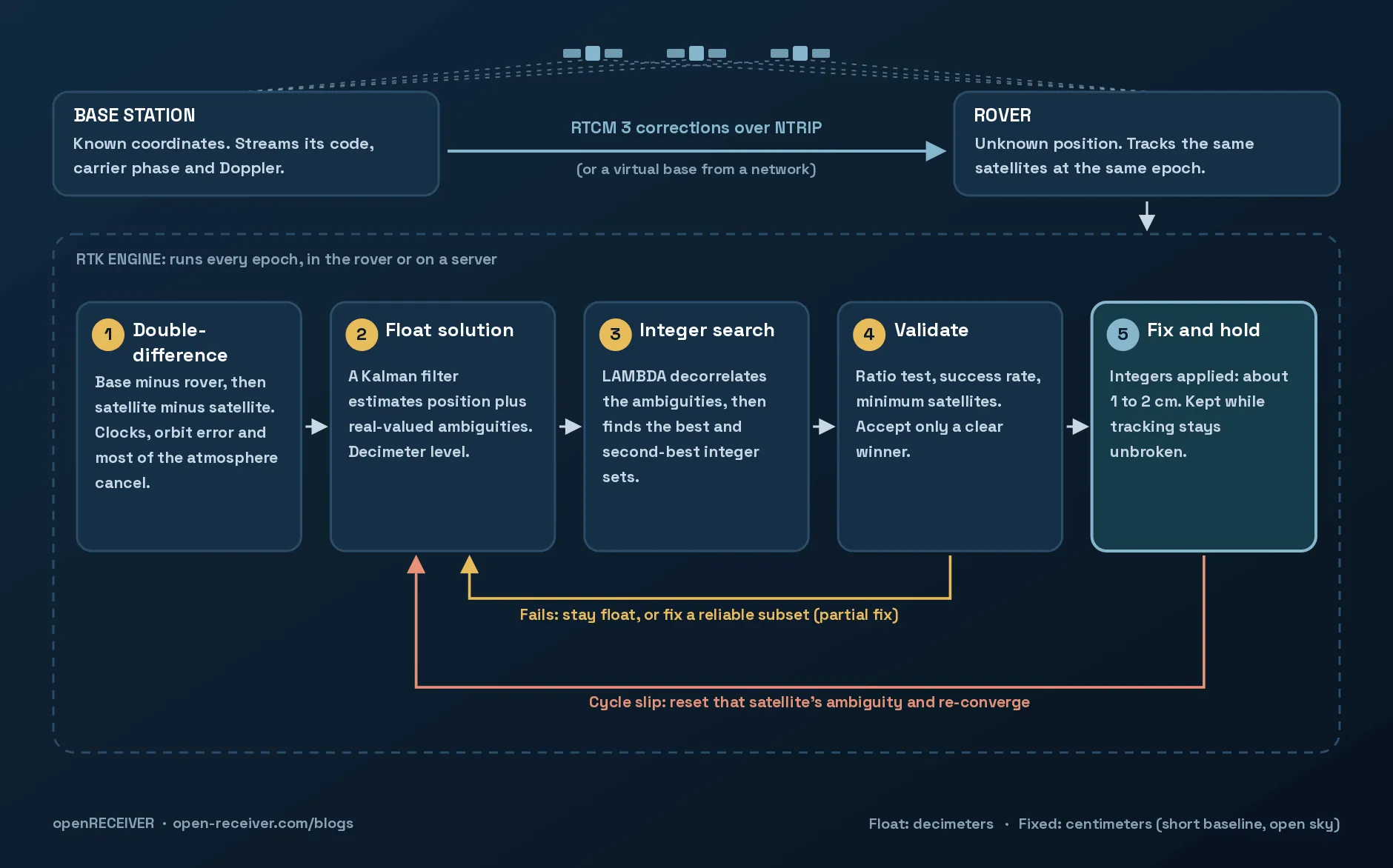Diagram of the RTK pipeline: a base station and a rover track the same satellites, RTCM 3 corrections flow over NTRIP, and the RTK engine runs double-differencing, float solution, LAMBDA integer search, validation, and fix-and-hold, with loops back for failed validation and cycle slips The RTK loop. Diagram: openRECEIVER.

Double-difference. Base minus rover, then satellite minus satellite. Clocks, orbit error and most of the atmosphere cancel. You literally substract the terms.
Float solution. A Kalman filter estimates position plus real-valued ambiguities. Decimeters.
Integer search. The Least-squares AMBiguity Decorrelation Adjustment (LAMBDA) method finds the best-fitting integer set and the runner-up.
Validate. Accept only a clear winner from a model strong enough to trust.
Fix and hold. Keep the integers (1 to 2 cm) until a cycle slip resets a satellite.

Why does RTK need the carrier phase?

According to the European Space Agency’s (ESA) Navipedia, the typical error of a code measurement is around 1 m, against about 5 mm for carrier phase. The problem is the unknown integer.

Picture a very very long tape measure with millimeter ticks, in 19 cm segements, with an unkonwn number of segements at your current position. The receiver reads its position within the last 19 cm segment (the Global Positioning System (GPS) L1 wavelength) almost perfectly, but not which segment it is in, like how many cycles alraedy traversed by the wave until it reached the receiver. That count is the integer ambiguity N, and one cycle wrong moves the range by 19 cm. RTK pins N.

phase (m) = range + c·(dt_receiver - dt_satellite) + troposphere - ionosphere
            + λ·N + hardware biases + multipath + noise

Step 1: what double-differencing cancels

Term	Base minus rover (single difference)	Then satellite minus satellite (double difference)
Satellite clock, satellite hardware bias	Cancel	Gone
Orbit error	Nearly cancels; residual grows with distance	Residual stays
Receiver clocks, receiver hardware bias	Remain	Cancel
Ionosphere, troposphere	Mostly cancel on short baselines; residual grows with distance	Residual stays
Multipath, receiver noise	Do not cancel; noise grows	Do not cancel; noise grows again
Ambiguity N	Remains	Remains, now a pure integer

The last row is why RTK can fix at all: with the fractional hardware biases gone, N is a true integer. PPP, with no base to difference against, needs externally estimated satellite phase biases to get there (PPP Ambiguity Resolution, PPP-AR).

The other rows set the limits. Multipath never cancels, so antenna siting is part of the error budget. Orbit and atmospheric residuals grow with distance, hence specs of a constant plus a ppm term (1 ppm is 1 mm per km of baseline). The U.S. National Geodetic Survey (NGS) real-time guidelines cite 1 cm + 1 ppm horizontal and 2 cm + 1 ppm vertical at one sigma, and cap single-base baselines at 10 km for their most precise survey class and 20 km for looser ones. Datasheets quoting circular error probable (CEP), a 50% statistic, look tighter for the same performance.

Steps 2 and 3: the float solution and the LAMBDA search

RTKLIB, the widely used open-source engine, is typical: an Extended Kalman Filter (EKF) carries rover position, velocity and one ambiguity per satellite and frequency. Unconstrained, the ambiguities come out as decimals: the float solution, good to decimeters.

Fixing means finding the integer vector nearest the float estimate, weighted by its covariance. Brute force fails because the ambiguities are strongly correlated, which makes the search space an extremely elongated ellipsoid (Navipedia). LAMBDA, introduced by Peter Teunissen in 1993, decorrelates them with an integer transformation, then searches the near-spherical result for the best and second-best integer sets.

The float covariance also predicts success before the search runs. Its ambiguity dilution of precision (ADOP) maps to the probability of fixing correctly: below about 0.12 cycles, the success rate exceeds 99.9% (Odijk and Teunissen, 2008). Since ADOP needs only geometry and the noise model, it works for planning too. If it is poor, no acceptance threshold rescues the fix; the model needs more satellites, frequencies or time.

Step 4: how does RTK know the fix is right?

The classic check is the ratio test (Euler and Schaffrin, 1991): the residual of the second-best integer set divided by that of the best. RTKLIB accepts a fix above a default of 3. A fixed threshold ignores model strength, so with few satellites a high ratio can still be wrong. Production engines add:

a fixed-failure-rate ratio test (Verhagen and Teunissen, 2013), whose threshold follows model strength to cap the wrong-fix probability: looser when the model is strong, stricter when it is weak;
gates on satellite count, elevation and predicted success rate;
partial ambiguity resolution, fixing only the reliable subset when the full set fails.

NGS notes that manufacturers quote 99.9% confidence in a correct on-the-fly fix, yet multipath still causes wrong fixes with height errors beyond 2 dm, with no specific indication on the data collector. A float is labeled as float; a wrong fix is labeled exactly like a right one. Hence NGS calls redundancy, re-observing points hours later under different satellite geometry, the single most important real-time procedure.

Step 5: holding the fix through cycle slips

Fix-and-hold feeds the integers back into the filter as constraints: steadier and quicker to re-fix, but a wrong fix becomes self-confirming. Continuous mode re-resolves every epoch and cannot inherit a bad hold. Instantaneous mode keeps no ambiguity memory and needs a strong multi-frequency, multi-GNSS model.

A cycle slip ends the hold for one satellite: tracking breaks (foliage, a passing truck, a dip in carrier-to-noise density ratio (C/N0)) and the count jumps by an unknown integer. Engines catch slips via the receiver’s loss-of-lock flag, jumps in the geometry-free (L1 minus L2) or Melbourne-Wübbena combinations, or disagreement with Doppler-predicted phase, then reset that satellite’s ambiguity. Per NGS, surviving integers speed the re-fix considerably; a complete loss of lock (under a bridge, say) starts from scratch.

Why dual-frequency and multi-GNSS RTK fix faster

Signal or combination	Wavelength
GPS L1 / Galileo E1	19.0 cm
GPS L2	24.4 cm
GPS L5 / Galileo E5a	25.5 cm
Wide-lane (L1 minus L2)	86.2 cm
Extra-wide-lane (L2 minus L5)	5.86 m

A longer wavelength makes a given range error a smaller fraction of a cycle, so the integer is easier to pin. Engines fix the wide-lane first and use it to constrain the 19 cm narrow-lane; a third frequency adds an extra-wide-lane step in front. The cost is noise, about six times L1 for the wide-lane according to NGS. The Melbourne-Wübbena combination cancels geometry, clocks, troposphere and first-order ionosphere, leaving the wide-lane integer plus hardware biases (which cancel in double differences) and code-dominated noise.

More constellations shrink the float covariance further: Teunissen, Odolinski and Odijk (2014) showed single-epoch RTK with combined GPS and BeiDou on short baselines.

RTK vs network RTK, Post-Processed Kinematic (PPK) and PPP

Method	Corrections	Typical accuracy	Time to centimeters	Coverage
Single-base RTK	Observation Space Representation (OSR), one base	~1 cm + 1 ppm horizontal	Seconds to minutes	10 to 20 km (NGS)
Network RTK	OSR modeled across reference stations	~1 cm, ppm term largely removed	Seconds to minutes	Stations up to ~50 to 70 km apart
PPK	Same math, after the fact	Like RTK	None (offline)	Like RTK
PPP	State Space Representation (SSR): orbits, clocks, biases	cm to dm	Many tens of minutes	Global
PPP with RTK-style ambiguity resolution (PPP-RTK)	SSR plus regional atmosphere	~cm	Much shorter than PPP	Where the atmosphere model exists

Network RTK interpolates orbit and atmospheric errors to the rover, which NGS says eliminates or drastically reduces the ppm term. A Virtual Reference Station (VRS) service needs a two-way link: the rover sends its position as a GGA fix-data sentence in National Marine Electronics Association (NMEA) format and receives a synthetic base next to it. The Master-Auxiliary Concept (MAC) broadcasts a master station’s corrections plus differences for its neighbors.

Frequently asked questions

How does RTK work?

A base station at a known position and a rover track the same satellites. The base streams its carrier-phase data, usually as RTCM 3 over NTRIP or by radio. The rover differences both data sets to cancel shared errors, resolves and validates the integer cycle count to each satellite, and outputs a 1 to 2 cm position.

How accurate is RTK?

A fixed solution on a short baseline typically gives about 1 cm horizontal and 2 cm vertical at one sigma, plus 1 mm per km from the base, per the manufacturer specifications cited by NGS. Float solutions are decimeter level. Multipath, an obstructed sky and long baselines degrade both, and a wrong fix can be decimeters off.

What is the difference between RTK float and fix?

A float solution estimates the carrier-phase ambiguities as real numbers and is accurate to decimeters. A fixed solution has resolved them to integers and passed validation, which brings accuracy to centimeters. The switch is discrete, not gradual, and a fix can still be wrong, which is why engines use ratio tests and success-rate gates.

How far can the rover be from the RTK base station?

NGS guidance caps single-base baselines at 10 km for its most precise survey class and 20 km for looser ones, because ionospheric and orbit errors stop cancelling with distance. Network RTK, with reference stations up to about 50 to 70 km apart according to Navipedia, and PPP-RTK extend coverage much further.

What is the difference between RTK and PPK?

Both use the same double-differenced carrier-phase mathematics. RTK resolves the integer ambiguities in real time from a live correction stream. Post-Processed Kinematic (PPK) logs base and rover data and resolves them afterward, processing forward and backward in time, and needs no live data link, which is why drone mapping often prefers it.

Can a smartphone do RTK?

Partly. Android exposes raw GNSS measurements, and phones whose chipsets report carrier phase (accumulated delta range, ADR) on dual-frequency L1/L5 can run an RTK engine on the device. Small, linearly polarized phone antennas suffer heavy multipath and frequent cycle slips, so phone RTK is far less reliable than a survey receiver.

Sources and further reading

Accuracy and baseline figures are typical values as of 2026 and depend on receiver, antenna, geometry and ionospheric conditions.